3 Applications of Generative Modelling in Machine Learning for Structured Data

Unstructured Data to Structured Data

Generative modelling for unstructured data has received a lot of attention in the last 5 years around the world with hundreds of papers published on different architectures. There has been a lot of attention to its applications among the developer communities with notable examples of GANs

• 18 Impressive Applications of Generative Adversarial Networks (GANs)
• GAN — Some cool applications of GAN
• Top 6 Impressive Real-World Applications Of GANs
  

Yet at the same time, generative modelling for structured data has received significantly less attention despite the business need being arguably much greater.

The business need is primarily driven by 2 core problems:

1. Large volumes of data with poor signal-to-noise ratio, and
2. Increasing data compliance regulations.
   

In this blogpost we share 3 valuable applications of generative modeling for structured data in machine learning.

Application 1: Automatic Data Upsampling and Bootstrapping for Backtesting and Cross-Validation

Datasets commonly contain fewer data points in some areas within their domain, and this can decrease model performance if not treated carefully. Generative models can be used to reshape datasets and upsample areas where the density is low. This is especially useful for imbalanced datasets and the so-called simulated data scenarios.

1.1 Imbalanced datasets

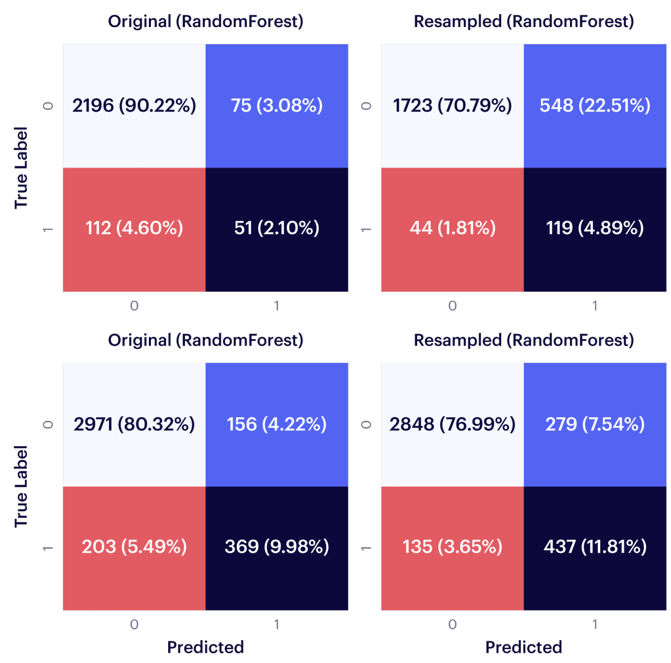
There are a few different techniques used to overcome this problem. One of the most commonly used is to oversample the dataset to obtain a new dataset with a balanced marginal distribution for the target class. The classifier is trained on the new dataset and the number of false negatives is drastically reduced. With a generative model, it’s possible to generate a new dataset that contains the desired distribution.

The confusion matrices below compare the performance of a Random Forest classifier trained on the original (imbalanced) dataset and a conditionally resampled dataset, for two different source datasets. As can be observed, false negatives decreased and true positives increased

1.2. Simulated Data Scenarios

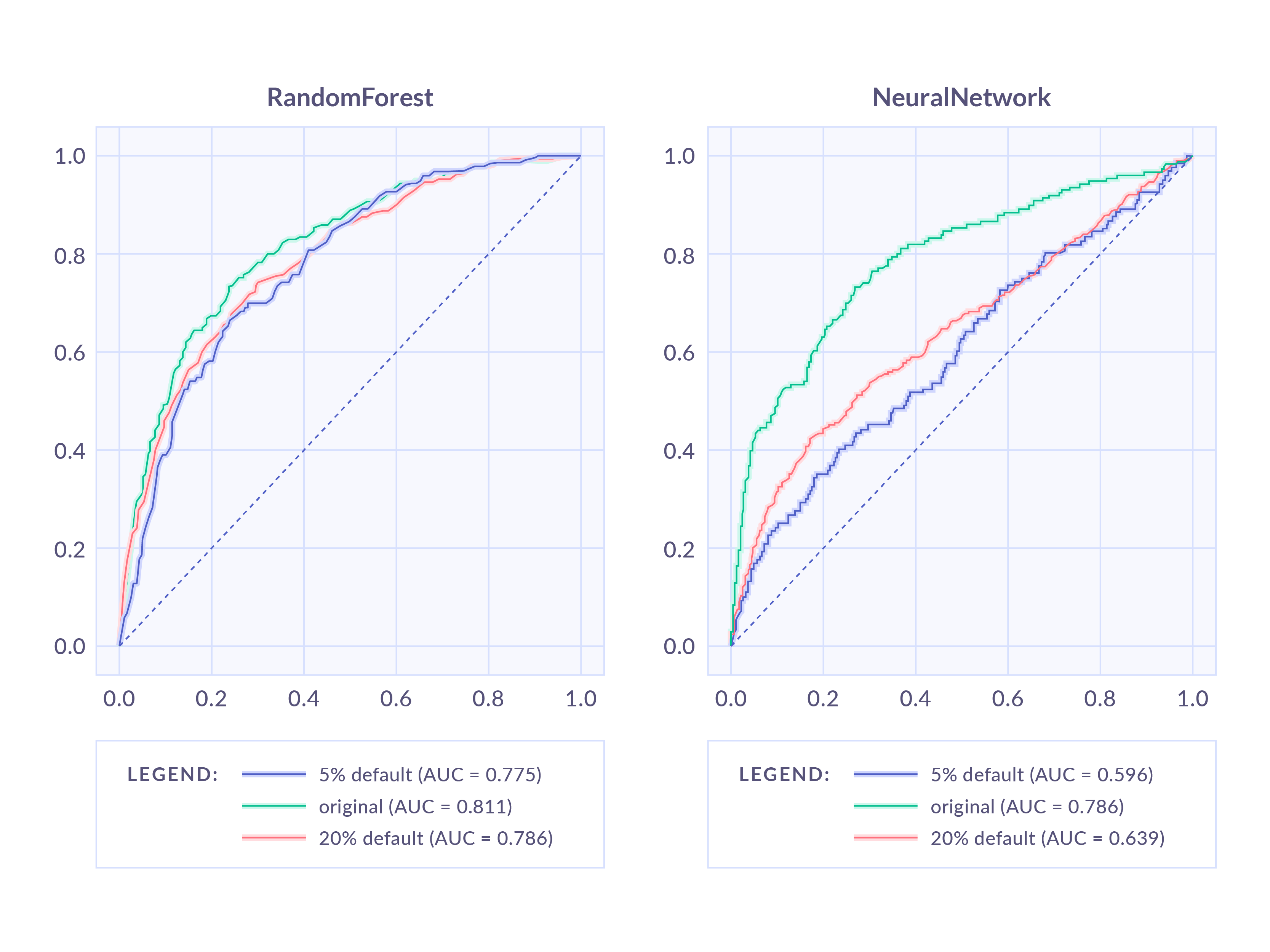
Another application of data reshaping is to modify distributions in the validation set, and quantify how robust a model is given population shifts and how it performs in different data segments. The goal is to answer questions such as “how does my model behave for younger and older users?” or “if due to unexpected circumstances the fraud rate is doubled next year, will my model still be able to detect this?”

In this case, a classifier is trained on the original data, and its performance is evaluated on different datasets created from a generative model. The image below shows the performance of a Random Forest and a Neural Network trained on the same dataset, but evaluated in three different scenarios. Although the Neural Network has better performance on the original set, the Random Forest is much more robust under population shifts.

Additional References:

• Data Science Applications of the Synthesized Platform
• Solving Data Imbalance with Synthetic Data
• Learning from Imbalanced Data‍
  

Application 2:  Data Imputation

Data acquisition processes are not perfect, which results in erroneous data points and missing values among other problems. General-purpose generative models can solve this problem by imputing data to values that have certain characteristics.

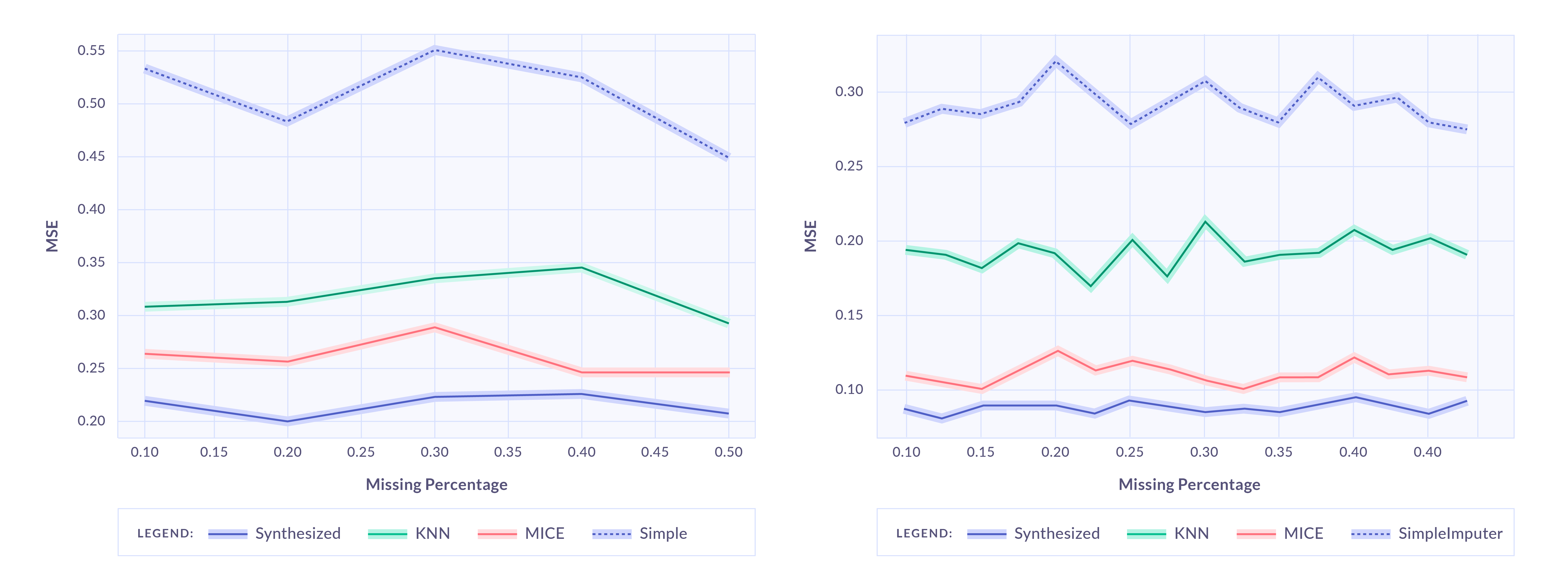
To do so, the information previously learned by the generative model is used to replace specific values with synthetic ones. The new values will keep the statistical information from the original dataset while the rest will be returned as they are. After imputing values, the user can directly use the whole dataset without having to remove it from outliers, missing values, or erroneous data.

There are different techniques to impute missing values. The figure below compares three of the most popular data imputation techniques (KNN, MICE and Simple Imputer; see references for more information) with data from a general-purpose generative model.

Additional References

• Imputation of missing values by Sklearn
• Van Buuren, Stef, and Karin Groothuis-Oudshoorn. "mice: Multivariate imputation by chained equations in R." Journal of statistical software 45.1 (2011): 1-67.
• Malarvizhi, R., and Antony Selvadoss Thanamani. "K-nearest neighbor in missing data imputation." International Journal of Engineering Research and Development 5.1 (2012): 5-7.

Application 3: Automatic Data Anonymization

Generative modelling enables powerful anonymisation of sensitive datasets whilst maintaining the utility that is often lost when applying classical anonymisation methods such as masking and grouping.

This approach to data anonymisation has a clear advantage compared to classical methods; your anonymised dataset no longer maintains the one-to-one mapping back to the original data as every row is generated by a generative model. This simple, yet powerful fact can significantly reduce the risk from data leakage when utilising sensitive datasets.

• If your data contains personal identifiable information (PII) such as names, addresses and bank details, it’s possible to generate realistic PII if required. This won’t just generate uncorrelated dummy data, but will accurately maintain the relationships between the PII fields. For example, if your dataset contains “gender”, “fullname”, “firstname” and “lastname” columns, these can be tied together to ensure the implicit relationship between them is preserved.

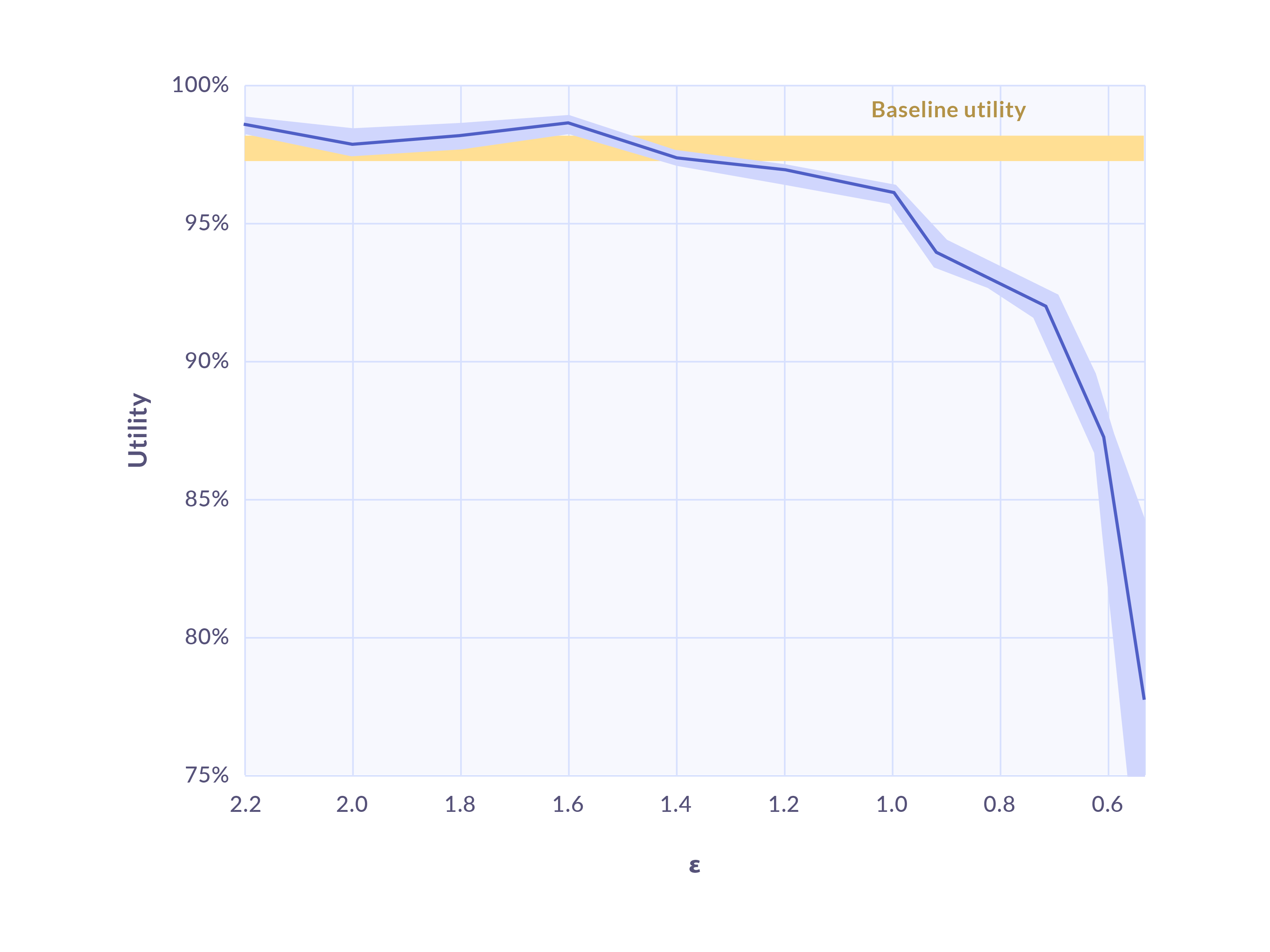
• Some generative models can also be configured for (ε,𝛿) differential privacy. This provides a mathematical guarantee of privacy by constraining the amount that individual rows within the original dataset can influence the generative model. This prevents the model from learning “too much” from original data and limits the influence of potentially risky outliers.  The figure above demonstrates the utility-privacy tradeoff as ε is decreased (increasing privacy) on an example dataset, where utility is measured as the performance of a machine learning classification task. Even with modest levels of differential privacy (ε=1.5), we can observe that the generated data can match the baseline utility of the original dataset.
  

Additional References:

• Classical Anonymisation Methods (K-anonymity)
• Differential Privacy
• Collaborating on Sensitive Data with Synthesized
  

The visualisations and examples mentioned within the blog post were created using the Synthesized SDK in Google Colab.